Module 4 - Merge Sort and Quick Sort

• 1. Understanding Merge Sort
• 2. Merge Sort in C++
• 3. Understanding Quick Sort
• 4. Lomuto Quick Sort in C++
• 5. Hoare Quick Sort in C++

1. Understanding Merge Sort

What is Merge Sort?

Merge Sort is an efficient, comparison-based sorting algorithm that uses a "divide and conquer" strategy. In simple terms, it repeatedly breaks down a list into several sub-lists until each sub-list contains only one item (which is considered sorted). Then, it merges those sub-lists back together in a sorted manner.

---

How Does it Work?

The process can be broken down into two main phases:

1. Divide Phase: The main, unsorted list is recursively divided in half. This continues until all the resulting sub-lists have only one element.
2. Conquer (Merge) Phase: Starting with the single-element lists, the algorithm repeatedly merges pairs of adjacent sub-lists. During each merge, it compares the elements from the two lists and combines them into a new, larger, sorted list. This continues until all the sub-lists have been merged back into a single, completely sorted list.

---

Visualization Explanation

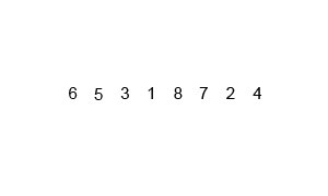
1. The Start: The animation begins with an unsorted list of numbers: [6, 5, 3, 1, 8, 7, 2, 4].

2. The "Divide" Phase:

   • First Split: The entire list is split into two halves: [6, 5, 3, 1] and [8, 7, 2, 4].
   • Second Split: Each of those halves is split again: [6, 5], [3, 1] and [8, 7], [2, 4].
   • Final Split: The splitting continues until we have eight separate lists, each containing just one number: [6], [5], [3], [1], [8], [7], [2], [4]. At this point, the "divide" phase is complete. A list with one item is inherently sorted.

3. The "Conquer (Merge)" Phase: Now, the algorithm starts merging these small lists back together in sorted order.

   • First Merge: It merges adjacent pairs. [5] and [6] are compared and merged to form [5, 6]. [1] and [3] are merged to form [1, 3]. Similarly, [7, 8] and [2, 4] are created. We now have four sorted sub-lists: [5, 6], [1, 3], [7, 8], and [2, 4].
   • Second Merge: The process repeats with these new, larger sorted lists. [5, 6] and [1, 3] are merged. The algorithm compares the first element of each list (1 vs 5), takes the 1, then compares 3 and 5, takes the 3

---

Benefits of Merge Sort

• Predictable Time Complexity: Its greatest strength is its consistent $O(n \log n)$ time complexity, regardless of the initial order of elements (worst, average, and best cases are the same). This makes it very reliable for large datasets.
• Stable Sort: Merge Sort is stable, meaning that if two elements have equal values, their relative order in the original array will be preserved in the sorted array.
• Excellent for External Sorting: It's highly effective for sorting data that is too large to fit into memory (e.g., files on a hard drive) because it reads and processes data in sequential chunks.
• Parallelizable: The "divide" step is easy to parallelize, meaning different parts of the array can be sorted simultaneously on different processor cores, speeding up the process significantly.

---

Drawbacks of Merge Sort

• Space Complexity: Its main disadvantage is that it requires extra space. It needs an auxiliary array of the same size as the input array, giving it a space complexity of O(n). This can be a limiting factor in memory-constrained environments like embedded systems.
• Slower for Small Datasets: For small lists, the overhead of recursion makes it slower than simpler algorithms like Insertion Sort. This is why many optimized sorting libraries use a hybrid approach.
• Recursive Overhead: The recursive function calls add some overhead to the execution stack, which, while usually minor, can be a consideration.

---

What is Merge Sort Used For?

Merge Sort's stability and efficiency with large datasets make it very useful in practice.

• Sorting Linked Lists: It is one of the most efficient ways to sort linked lists. Unlike arrays, linked lists are not easily accessible by index, but merging them is a very efficient operation.
• External Sorting: As mentioned, it's a go-to algorithm for sorting massive files that don't fit in RAM.
• Inversion Count Problem: The algorithm can be modified to solve other problems, such as counting the number of inversions in an array efficiently.
• Standard Library Implementations: It forms the basis of many highly optimized, built-in sorting functions in various programming languages, often as part of a hybrid algorithm like Timsort (used in Python and Java), which combines Merge Sort with Insertion Sort.

2. Merge Sort in C++

This section explains how the "divide and conquer" strategy of Merge Sort is implemented in C++. The logic is split into two primary functions: mergeSort() which handles the recursive division, and merge() which handles the conquering and sorting.

The C++ Code Implementation

Here is the complete code for a Merge Sort implementation using std::vector.

#include <iostream>
#include <vector>

// Utility function to print a vector
void printVector(const std::vector<int>& arr) {
    for (int num : arr) {
        std::cout << num << " ";
    }
    std::cout << std::endl;
}

// Merges two sorted subarrays into a single sorted subarray.
// First subarray is arr[left..mid]
// Second subarray is arr[mid+1..right]
void merge(std::vector<int>& arr, int left, int mid, int right) {
    // Calculate sizes of the two temporary subarrays
    int n1 = mid - left + 1;
    int n2 = right - mid;

    // Create temporary vectors to hold the data
    std::vector<int> L(n1), R(n2);

    // Copy data from the main array to the temporary vectors
    for (int i = 0; i < n1; i++)
        L[i] = arr[left + i];
    for (int j = 0; j < n2; j++)
        R[j] = arr[mid + 1 + j];

    // Merge the temporary vectors back into the original array arr[left..right]
    int i = 0; // Initial index for left subarray
    int j = 0; // Initial index for right subarray
    int k = left; // Initial index for the merged subarray

    while (i < n1 && j < n2) {
        if (L[i] <= R[j]) {
            arr[k] = L[i];
            i++;
        } else {
            arr[k] = R[j];
            j++;
        }
        k++;
    }

    // Copy any remaining elements from the left subarray
    while (i < n1) {
        arr[k] = L[i];
        i++;
        k++;
    }

    // Copy any remaining elements from the right subarray
    while (j < n2) {
        arr[k] = R[j];
        j++;
        k++;
    }
}

// The main recursive function that implements the "divide" phase
void mergeSort(std::vector<int>& arr, int left, int right) {
    // Base case: if the array has 1 or 0 elements, it's already sorted
    if (left >= right) {
        return;
    }

    // Find the middle point to divide the array
    int mid = left + (right - left) / 2;

    // Recursively call mergeSort for the two halves
    mergeSort(arr, left, mid);
    mergeSort(arr, mid + 1, right);

    // Merge the two now-sorted halves
    merge(arr, left, mid, right);
}

// Main driver function
int main() {
    std::vector<int> data = {6, 5, 3, 1, 8, 7, 2, 4};
    std::cout << "Original array: ";
    printVector(data);

    mergeSort(data, 0, data.size() - 1);

    std::cout << "Sorted array:   ";
    printVector(data);

    return 0;
}

Output

Original array: 6 5 3 1 8 7 2 4 
Sorted array:   1 2 3 4 5 6 7 8 

Code Breakdown

---

Code Breakdown

The mergeSort() Function: The Divider

This function is the engine that drives the "Divide" phase.

1. Base Case: The recursion stops when left >= right, which means the sub-array has one or zero elements and is considered sorted.
2. Divide: It calculates the mid point of the current array segment. The formula left + (right - left) / 2 is used to prevent potential overflow on very large arrays.
3. Recurse: It calls itself for the left half (left to mid) and then for the right half (mid + 1 to right).
4. Conquer: After the recursive calls return (guaranteeing the two halves are sorted), it calls merge() to combine them into a single, sorted segment.

The merge() Function: The Conqueror

This function is the core of the algorithm where the actual sorting happens. It takes two adjacent, sorted sub-arrays and merges them.

1. Setup: It creates two temporary vectors, L and R, and copies the data from the two halves of the main array into them.
2. Merge Loop: It uses three index pointers: i for vector L, j for vector R, and k for the original array arr. It compares the elements at L[i] and R[j] and places the smaller of the two into arr[k]. It then increments the pointer of the vector from which the element was taken, as well as the pointer k.
3. Copy Leftovers: After the main loop, one of the temporary vectors might still contain elements. The final two while loops copy these remaining elements back into the main array, ensuring all data is merged correctly.

3. Understanding Quick Sort

What is Quick Sort?

Quick Sort is a highly efficient, comparison-based sorting algorithm that also uses a "divide and conquer" strategy. It is one of the most widely used sorting algorithms due to its fast average-case performance. The core idea is to select a 'pivot' element from the array and partition the other elements into two sub-arrays, according to whether they are less than or greater than the pivot. The sub-arrays are then sorted recursively.

---

How Does it Work?

The process can be broken down into three main steps:

1. Pivot Selection: Choose an element from the array to be the pivot. Common strategies include picking the first element, the last element, the middle element, or a random element.

2. Partitioning: Reorder the array so that all elements with values less than the pivot are on one side, and all elements with values greater than the pivot are on the other. This crucial step can be performed in several ways, with the two most common being:

   • Lomuto Partition Scheme: This is a very intuitive method. It typically uses the last element as the pivot. It then scans the array with a single pointer, maintaining a "wall" that separates smaller elements from the rest. After the scan, the pivot is swapped into its final, sorted position. This scheme is easy to implement but can be inefficient with already-sorted data.

   • Hoare Partition Scheme: This is the original method and is generally faster. It often uses the first element as the pivot. It uses two pointers—one at each end of the array—that move toward each other, swapping elements as they go. This method correctly separates the values, but the pivot itself does not necessarily end up in its final sorted position.

3. Recursion: Recursively apply the above steps to the sub-arrays on both sides of the partition. This continues until the base case of an array with zero or one element is reached, at which point the entire array is sorted.

---

Visualization Explanation

Lomuto Partition Scheme

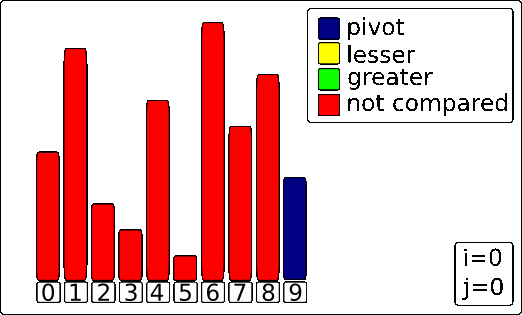
The algorithm uses three key components, which are represented by colors in the animation:

• The Pivot (blue bar): The value everything else is compared against. In this scheme, it's the last element.
• The Scanner j (yellow highlight): This pointer moves through the array to inspect each element.
• The Wall i (green highlight): This pointer marks the boundary for elements that are smaller than the pivot.

The Process

Here's a step-by-step breakdown of the process shown in the GIF.

1. The Setup

The process begins by selecting the last element of the array as the Pivot (making it blue). The Wall (i) is placed just before the first element, and the Scanner (j) starts at the first element.

2. The Partitioning Loop

The Scanner (j) moves from left to right, one element at a time. For each element it inspects, one of two things happens:

• If the element is LARGER than the Pivot: The element is already on the "correct" side of where the pivot will eventually be. The algorithm does nothing but advance the Scanner j to the next element.

• If the element is SMALLER than the Pivot: This is the key action. The algorithm needs to move this smaller element to the left section of the array. It does this in two steps:

  1. The Wall (i) is moved one position to the right to make room in the "smaller than pivot" section.
  2. The smaller element at the Scanner's position (j) is swapped with the element now at the Wall's new position (i).

This loop continues until the Scanner has inspected every element except for the pivot itself.

3. Final Pivot Placement

After the loop finishes, all elements smaller than the pivot are now grouped together on the left side of the Wall. The final step is to place the pivot in its correct sorted position.

This is done by swapping the Pivot (the blue bar) with the element that is immediately to the right of the Wall (i+1).

The result is a perfectly partitioned array. The pivot is now in its final place, with every element to its left being smaller and every element to its right being larger. This process is then repeated recursively on the sub-arrays to the left and right of the pivot.

Hoare Partition Scheme

How It Works: A Breakdown

Here’s a breakdown of the process for any given array segment.

1. The Setup

• Pivot Selection: An element is chosen as the pivot. In this animation, it appears to be the first element of the segment being sorted.
• Two Pointers: Two pointers are established: a left pointer i and a right pointer j, starting at opposite ends of the segment.

2. The Partitioning Loop ↔️

This is the main action you see in the animation. The two pointers begin moving towards the center of the array to find elements that are on the wrong side of the pivot.

1. The left pointer i moves to the right, skipping over all elements that are smaller than the pivot. It stops when it finds an element larger than or equal to the pivot.
2. The right pointer j moves to the left, skipping over all elements that are larger than the pivot. It stops when it finds an element smaller than or equal to the pivot.
3. The Swap: Once both pointers have stopped, if they haven't crossed each other, the two elements they are pointing at are swapped. This places both elements on their correct side of the partition.

This search-and-swap process repeats until the pointers cross.

3. The Result

When the pointers cross, the loop terminates. The array segment is now partitioned into two groups:

• A left partition where all values are less than or equal to the pivot's value.
• A right partition where all values are greater than or equal to the pivot's value.

Crucially, unlike other methods, the pivot itself does not necessarily end up in its final sorted position. The algorithm then recursively repeats this entire process on the two new sub-arrays.

---

Benefits of Quick Sort

• Fast on Average: It has an average-case time complexity of O(n log n), which is extremely fast in practice, often outperforming other sorting algorithms.
• In-place Sorting: It has a space complexity of O(log n) on average because it sorts the array "in-place," meaning it doesn't require a separate auxiliary array like Merge Sort.
• Low Overhead: The inner loop of the algorithm is very simple and can be implemented efficiently on most machine architectures.

---

Drawbacks of Quick Sort

• Worst-Case Performance: Its main weakness is a worst-case time complexity of O(n^2). This occurs when the chosen pivots are consistently the smallest or largest elements, which can happen with already-sorted or reverse-sorted data.
• Unstable Sort: Quick Sort is unstable. It does not guarantee that the relative order of equal elements will be preserved after sorting.
• Sensitive to Pivot Choice: The efficiency of the algorithm is highly dependent on the pivot selection strategy. A

4. Lomuto Quick Sort in C++

This section explains how the "divide and conquer" strategy of Quick Sort is implemented in C++. The logic is split into two primary functions: quickSort() which handles the recursive division, and partition() which rearranges the array using the popular Lomuto partition scheme.

The C++ Code Implementation

Here is the complete code for a Quick Sort implementation using std::vector.

#include <iostream>
#include <vector>
#include <utility> // For std::swap

// Utility function to print a vector
void printVector(const std::vector<int>& arr) {
    for (int num : arr) {
        std::cout << num << " ";
    }
    std::cout << std::endl;
}

// This function implements the Lomuto partition scheme. It takes the last 
// element as pivot and places it at its correct position in the sorted array.
int partition(std::vector<int>& arr, int low, int high) {
    // Choose the last element as the pivot (key to Lomuto)
    int pivot = arr[high]; 
    
    // Index of the smaller element, acting as a "wall"
    int i = (low - 1); 

    for (int j = low; j <= high - 1; j++) {
        // If the current element is smaller than the pivot
        if (arr[j] < pivot) {
            i++; // Move the wall to the right
            std::swap(arr[i], arr[j]);
        }
    }
    // Place the pivot in its correct position after the wall
    std::swap(arr[i + 1], arr[high]);
    return (i + 1);
}

// The main recursive function that implements Quick Sort
void quickSort(std::vector<int>& arr, int low, int high) {
    // Base case: if the array has 1 or 0 elements, it's already sorted
    if (low < high) {
        // pi is the partitioning index from the Lomuto partition
        int pi = partition(arr, low, high);

        // Separately sort elements before and after the partition
        quickSort(arr, low, pi - 1);
        quickSort(arr, pi + 1, high);
    }
}

// Main driver function
int main() {
    std::vector<int> data = {6, 5, 3, 1, 8, 7, 2, 4};
    std::cout << "Original array: ";
    printVector(data);

    quickSort(data, 0, data.size() - 1);

    std::cout << "Sorted array:   ";
    printVector(data);

    return 0;
}

Output

Original array: 6 5 3 1 8 7 2 4 
Sorted array:   1 2 3 4 5 6 7 8 

Code Breakdown

The quickSort() Function: The Recursive Driver

This function orchestrates the "Divide" phase of the algorithm.

1. Base Case: The recursion continues as long as low < high. If low >= high, it means the sub-array has one or zero elements, which is inherently sorted.
2. Partition: It calls the partition() function. This function rearranges the sub-array and returns the index pi where the pivot element is now correctly placed.
3. Recurse: It calls itself twice for the two sub-arrays created by the partition: one for the elements to the left of the pivot (low to pi - 1) and one for the elements to the right (pi + 1 to high). Because this uses the Lomuto scheme, the pivot at pi is guaranteed to be in its final place and can be excluded from recursion.

The partition() Function (Lomuto Scheme)

This function implements the well-known Lomuto partition scheme. It is where the key logic of rearranging elements occurs and can be seen as the "Conquer" step, as it correctly places one element (the pivot) at a time.

1. Pivot Selection: It selects the last element of the sub-array (arr[high]) as the pivot. This is the defining starting point for this version of Lomuto.
2. Rearranging Loop: It maintains an index i (the "wall") which represents the boundary for elements smaller than the pivot. It iterates through the sub-array with another index j (the "scanner"). If it finds an element arr[j] that is smaller than the pivot, it moves the wall (i++) and swaps arr[j] with the element at the new wall position, effectively expanding the "smaller than pivot" section.
3. Final Pivot Placement: After the loop finishes, all elements smaller than the pivot are at the beginning of the sub-array. The pivot (still at arr[high]) is then swapped with the element at arr[i + 1]. This places the pivot exactly where it belongs in the sorted array.
4. Return Index: The function returns the new index of the pivot (i + 1), so the quickSort function knows where to split the array for its next recursive calls.

5. Hoare Quick Sort in C++

This section explains how the "divide and conquer" strategy of Quick Sort is implemented in C++. The logic is split into two primary functions: quickSort() which handles the recursive division, and partition() which rearranges the array using the classic Hoare partition scheme.

The C++ Code Implementation

Here is the complete code for a Quick Sort implementation using the Hoare partition scheme.

#include <iostream>
#include <vector>
#include <utility> // For std::swap

// Utility function to print a vector
void printVector(const std::vector<int>& arr) {
    for (int num : arr) {
        std::cout << num << " ";
    }
    std::cout << std::endl;
}

// This function implements the Hoare partition scheme. It partitions the
// array and returns the split point.
int partition(std::vector<int>& arr, int low, int high) {
    // Choose the first element as the pivot (key to this Hoare implementation)
    int pivot = arr[low];
    int i = low - 1;
    int j = high + 1;

    while (true) {
        // Find an element on the left side that should be on the right
        do {
            i++;
        } while (arr[i] < pivot);

        // Find an element on the right side that should be on the left
        do {
            j--;
        } while (arr[j] > pivot);

        // If the pointers have crossed, the partition is done
        if (i >= j) {
            return j;
        }

        // Swap the elements to place them on the correct side
        std::swap(arr[i], arr[j]);
    }
}

// The main recursive function that implements Quick Sort
void quickSort(std::vector<int>& arr, int low, int high) {
    // Base case: if the array has 1 or 0 elements, it's already sorted
    if (low < high) {
        // pi is the split point from the Hoare partition
        int pi = partition(arr, low, high);

        // Recursively sort the two partitions
        quickSort(arr, low, pi);
        quickSort(arr, pi + 1, high);
    }
}

// Main driver function
int main() {
    std::vector<int> data = {6, 5, 3, 1, 8, 7, 2, 4};
    std::cout << "Original array: ";
    printVector(data);

    quickSort(data, 0, data.size() - 1);

    std::cout << "Sorted array:   ";
    printVector(data);

    return 0;
}

Output

Original array: 6 5 3 1 8 7 2 4 
Sorted array:   1 2 3 4 5 6 7 8 

Code Breakdown

The quickSort() Function: The Recursive Driver

This function orchestrates the "Divide" phase of the algorithm.

1. Base Case: The recursion continues as long as low < high. If low >= high, it means the sub-array has one or zero elements.
2. Partition: It calls the partition() function, which rearranges the sub-array and returns a split point index pi.
3. Recurse: It calls itself on the two partitions. Because the Hoare scheme's split point pi is not guaranteed to be the pivot's final position, the recursive calls are quickSort(arr, low, pi) and quickSort(arr, pi + 1, high) to ensure all elements are included in the sorting process.

The partition() Function (Hoare Scheme)

This function implements the classic Hoare partition scheme. It is generally more efficient than Lomuto because it performs fewer swaps on average.

1. Pivot Selection: It selects the first element (arr[low]) as the pivot.
2. Two Pointers: It uses two pointers, i and j, which start at opposite ends of the array and move toward each other.
3. Rearranging Loop: The i pointer moves right to find the first element greater than or equal to the pivot, while the j pointer moves left to find the first element less than or equal to the pivot. If the pointers haven't crossed, the two elements are swapped.
4. Return Index: The loop terminates when the pointers cross. The function returns the final position of the j pointer, which serves as the split point for the two partitions. Unlike Lomuto, the pivot is not guaranteed to be at this returned index.