3. Understanding Quick Sort

What is Quick Sort?

Quick Sort is a highly efficient, comparison-based sorting algorithm that also uses a "divide and conquer" strategy. It is one of the most widely used sorting algorithms due to its fast average-case performance. The core idea is to select a 'pivot' element from the array and partition the other elements into two sub-arrays, according to whether they are less than or greater than the pivot. The sub-arrays are then sorted recursively.

How Does it Work?

The process can be broken down into three main steps:

Pivot Selection: Choose an element from the array to be the pivot. Common strategies include picking the first element, the last element, the middle element, or a random element.
Partitioning: Reorder the array so that all elements with values less than the pivot are on one side, and all elements with values greater than the pivot are on the other. This crucial step can be performed in several ways, with the two most common being:
- Lomuto Partition Scheme: This is a very intuitive method. It typically uses the last element as the pivot. It then scans the array with a single pointer, maintaining a "wall" that separates smaller elements from the rest. After the scan, the pivot is swapped into its final, sorted position. This scheme is easy to implement but can be inefficient with already-sorted data.
- Hoare Partition Scheme: This is the original method and is generally faster. It often uses the first element as the pivot. It uses two pointers—one at each end of the array—that move toward each other, swapping elements as they go. This method correctly separates the values, but the pivot itself does not necessarily end up in its final sorted position.
Recursion: Recursively apply the above steps to the sub-arrays on both sides of the partition. This continues until the base case of an array with zero or one element is reached, at which point the entire array is sorted.

Visualization Explanation

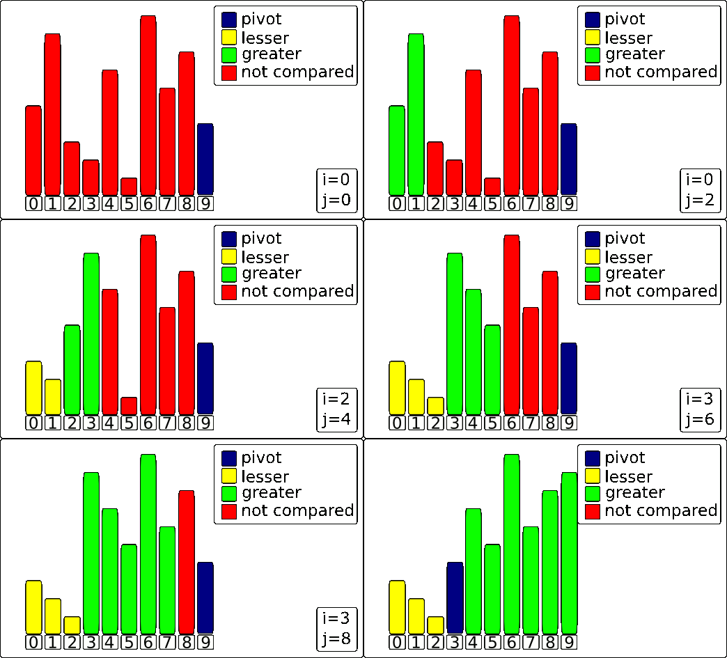
Lomuto Partition Scheme

~~Of course. This GIF provides an excellent visual for how the Lomuto partition scheme works. It's the core engine of one of the most common Quick Sort implementations.~~

The algorithm uses three key components, which are represented by colors in the animation:

The Pivot (blue bar): The value everything else is compared against. In this scheme, it's the last element.
The Scanner j (yellow highlight): This pointer moves through the array to inspect each element.
The Wall i (green highlight): This pointer marks the boundary for elements that are smaller than the pivot.

The Process

Here's a step-by-step breakdown of the process shown in the GIF.

1. The Setup

The process begins by selecting the last element of the array as the Pivot (making it blue). The Wall (i) is placed just before the first element, and the Scanner (j) starts at the first element.

2. The Partitioning Loop

The Scanner (j) moves from left to right, one element at a time. For each element it inspects, one of two things happens:

If the element is LARGER than the Pivot: The element is already on the "correct" side of where the pivot will eventually be. The algorithm does nothing but advance the Scanner j to the next element.
If the element is SMALLER than the Pivot: This is the key action. The algorithm needs to move this smaller element to the left section of the array. It does this in two steps:
1. The Wall (i) is moved one position to the right to make room in the "smaller than pivot" section.
2. The smaller element at the Scanner's position (j) is swapped with the element now at the Wall's new position (i).

This loop continues until the Scanner has inspected every element except for the pivot itself.

3. Final Pivot Placement

After the loop finishes, all elements smaller than the pivot are now grouped together on the left side of the Wall. The final step is to place the pivot in its correct sorted position.

This is done by swapping the Pivot (the blue bar) with the element that is immediately to the right of the Wall (i+1).

The result is a perfectly partitioned array. The pivot is now in its final place, with every element to its left being smaller and every element to its right being larger. This process is then repeated recursively on the sub-arrays to the left and right of the pivot.

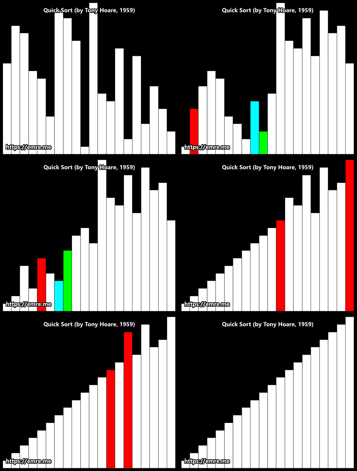
Hoare Partition Scheme

How It Works: A Breakdown

Here’s a breakdown of the process for any given array segment.

1. The Setup

Pivot Selection: An element is chosen as the pivot. In this animation, it appears to be the first element of the segment being sorted.

Two Pointers: Two pointers are established: a left pointer i and a right pointer j, starting at opposite ends of the segment.

2. The Partitioning Loop ↔️

This is the main action you see in the animation. The two pointers begin moving towards the center of the array to find elements that are on the wrong side of the pivot.

The left pointer i moves to the right, skipping over all elements that are smaller than the pivot. It stops when it finds an element larger than or equal to the pivot.

The right pointer j moves to the left, skipping over all elements that are larger than the pivot. It stops when it finds an element smaller than or equal to the pivot.

The Swap: Once both pointers have stopped, if they haven't crossed each other, the two elements they are pointing at are swapped. This places both elements on their correct side of the partition.

This search-and-swap process repeats until the pointers cross.

3. The Result

When the pointers cross, the loop terminates. The array segment is now partitioned into two groups:

A left partition where all values are less than or equal to the pivot's value.

A right partition where all values are greater than or equal to the pivot's value.

Crucially, unlike other methods, the pivot itself does not necessarily end up in its final sorted position. The algorithm then recursively repeats this entire process on the two new sub-arrays.

Benefits of Quick Sort

Fast on Average: It has an average-case time complexity of O(n log n), which is extremely fast in practice, often outperforming other sorting algorithms.
In-place Sorting: It has a space complexity of O(log n) on average because it sorts the array "in-place," meaning it doesn't require a separate auxiliary array like Merge Sort.
Low Overhead: The inner loop of the algorithm is very simple and can be implemented efficiently on most machine architectures.

Drawbacks of Quick Sort

Worst-Case Performance: Its main weakness is a worst-case time complexity of O(n^2). This occurs when the chosen pivots are consistently the smallest or largest elements, which can happen with already-sorted or reverse-sorted data.
Unstable Sort: Quick Sort is unstable. It does not guarantee that the relative order of equal elements will be preserved after sorting.
Sensitive to Pivot Choice: The efficiency of the algorithm is highly dependent on the pivot selection strategy. A